SWING, Small and Wide angle X-ray scattering
Pour l'étude d'échantillons à structure complexe : macromolécules, nanomatériaux, tissus...
Pour plus d'informations, merci de vister le site en anglais
For more informations, please visit the english website
Fournissant des informations sur la structure de la matière à des échelles comprises entre le nanomètre et le micromètre, la ligne SWING permettra de répondre aux nombreuses questions liées à la matière molle, à la conformation de macromolécules en solution et aux matières composites en sciences des matériaux.
Cette installation expérimentale permettra d'effectuer simultanément des mesures de diffusion de rayons X aux petits angles (SAXS) et grands angles (WAXS) dans la gamme d'énergie de 5-16 keV aussi bien que des mesures de diffusion en incidence rasante (GISAXS). Des expériences de diffusion anomale seront également possibles. L'accent sera mis sur la variété d'échantillons qui peuvent être étudiés, solutions, gels, solides amorphes, solides cristallisés et sur la diversité des environnements correspondants.
L'équipe
Nos dernières publications sur twitter
-
Données techniques
Between ~5 and 16 keV
~2 eV
In-vacuum U20 undulator.
Source Size (sigma, μm): 388 (H) x 8.1 (V)
Source Divergence (sigma, μrad): 14.5 (H) x 4.6 (V)
Diaphragm at 11.7 m (1x0.5 mm2)
Fixed exit DCM Si111at 20 m
Fixed incidence focusing KB at 22.5 m
Sample position : 30 - 32 m
Detector / Sample Distance : 0.5 – 6.5 m
see Set-up environments
Between 20x20µm2 (zone plate) to 450x20 μm2 FWHM in the experimental hutch
1.1013ph/s @7keV, 1.1012 ph/s @16keV (with 500 mA ring)
SAXS:
- Eiger 4M (Dectris)
- PCCD170170 (AVIEX), Gain > 3ADU/ph, Noise≈2ADU
WAXS:
- Hybrid Pixel detector (Detector Group pool)
Under primary vacuum, SAXS detector positions :
- 0.20 / + 0. 20 m (horiz), -0.20 / +0.20 (vert), 0.5 m / +6 m (along X-rays).
Dedicated sample environments have been developed to provide scientific communities with optimized experimental conditions. For soft-condensed matter, numerous devices are available (home-made capillaries holders, Linkam THMS600, Anton Paar rheometer with custom-made Couette cells …). For structural biology, a unique SEC-SAXS HPLC system is routinely used for online purification connected to a quartz capillary placed under vacuum cell. Here are presented the most used devices for both soft-condensed matter and structural biology.
HPLC: SEC-SAXS
 |
|
AutoSampler for BioSaxs
 |
|
High Pressure
description will arrive soon
Static Capillaries Holder
|
|
|
Circulation Capillaries Holder
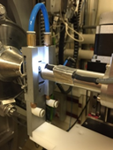 |
Circulation through the capillaries can be done using various setups :
|
Gel Holder
description will arrive soon
Mixing and pipetting cell
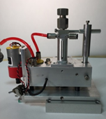 |
The sample is drawn in the capillary only and at the required height. After X-ray exposition, it’s reinjected into the mixing cell. |
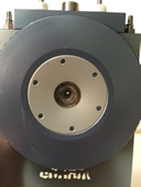
Linkam
 |
|
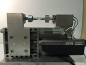
Traction Cell
 |
|
Rheometer
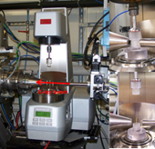 |
Rheometer Anton Paar MCR 501
|
Stop-Flow (+MALS)
description will arrive soon
Micro-fluidic
description will arrive soon
BioSaxs
Before Coming
What you have to bring
We use Agilent standards vials and inserts for the HPLC device and the Auto Sampler. We lend you the vials and the caps but you have to buy you own inserts (Agilent reference: 5181-1270). In any case, we can give some used inserts that you can wash and dry.
The minimum quantity of buffer is 40ml for one injection (10mL of system purge + 20 mL of column equilibration + 10mL of elution). We will recommande you to bring much more (100mL to 500mL) to obtain a better equilibration of the column and to induce less stress in case of trouble.
To make your backups directly on the line, a Windows compatible hard disk is required. However, you can still download all your data a posteriori via the sunset[Experiment Data][Soleil Data Retrivial].
What we can lend you
The biology laboratory (link) provides support to users for the preparation of their experiments. For any question, please ask the laboratory staff.
We recommend you to bring your own analytical columns for SEC-SAXS. We have also a wide selection of column for users. All these columns have been calibrated:
|
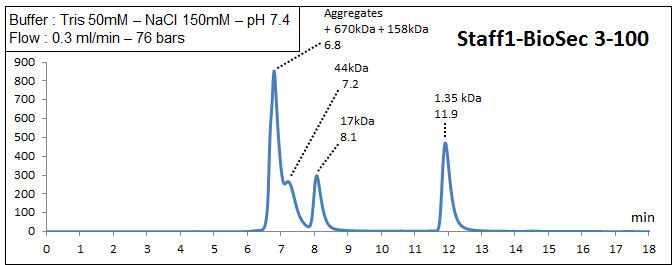
BioSec3-100 Column Volume:5mL Mass Range: 0.1 to 100kDa pH Range: 2-8.5 |
 |
|
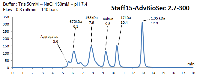
AdvBioSec 2.7-300 Column Volume:5mL Mass Range: 5 to 1250kDa pH Range: 2-8.5 |
 |
|
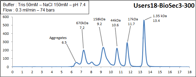
BioSec3-300 Column Volume:5mL Mass Range: 5 to 1250kDa pH Range: 2-8.5 |
 |
|
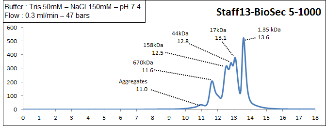
BioSec 5-1000 Column Volume:5mL Mass Range: 50 to 7500kDa pH Range: 2-8.5 |
 |
|
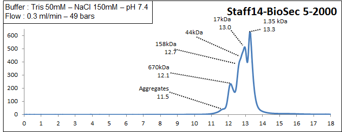
BioSec 5-2000 Column Volume:5mL Mass Range: >10000kDa pH Range: 2-8.5 |
 |
During your session
The session includes beamline set up installation. It’s recommended to discuss with your local contact before coming to the beamline to save time during installation.
Running experiments
Our GUI (passerelle) allows automatic data collections of multiples simple in a row. For direct data monitoring and security check, an others GUI (Cook) is installed.
The local contact will show you how to use these GUI.
Data Processing and analysis: Foxtrot & AutoBioSAXS
All the images produced on the Swing beamline can be process by homemade software (Foxtrot) in collaboration with Xenocs. You can ask for it by email to Xenocs by mail.
You can find here (new link) a tutorial for processing SEC-SAXS experiments.
For SEC-SAXS and BioSaxs AutoSampler, an automatic workflow for data analysis is available. This workflow takes raw images as input files and sends all results curves into IspyB database. Furthermore all intermediates files are available for users and could be reloading in our Foxtrot application.
Living area
We have a living area where you can use coffee machine, Sofa, fridge for food and beverages, micro wave and table. Wifi is available using your sunset login and password or using Eduroam network.
This area is sample free and please clean it after your session.
After your session
Please don’t forget to fill the end of report in the sunset webpage.
All your datas are available using the Soleil data Retrieval via the sunset web page.
ChemSaxs
During your session
The session includes beamline set up installation. It’s recommended to discuss with your local contact before coming to the beamline to save time during installation.
Running experiments
Our GUI (passerelle) allows an “on demand” complex data collections strategies. For most of the sample environment, a workflow is already written. For direct data monitoring and security check, an others GUI (Cook) is installed. The local contact will show you how to use these GUI.
Data Processing and analysis: Foxtrot & AutoChemSAXS
All the images produced on the Swing beamline can be process by homemade software in collaboration with Xenocs. You can ask for it by email to Xenocs (link).
Living area
We have a living area where you have coffee machine, Sofa, fridge for food and beverages, micro wave and table. Wifi is available using your sunset login and password or using Eduroam network.
This area is sample free and please cleans it after your session.
After your session
Please don’t forget to fill the end of report in the sunset webpage.
All your datas are available using the Soleil data Retrieval via the sunset web page.
en cours...
en cours...
Listes des logiciels développés par la ligne SWING.
Programme Foxtrot
Programme Foxtrot (Réduction et analyse des données)
Demande par mail
Tutoriel pour Foxtrot :
Foxtrot : F.A.Q.
Programme Denfert
Programme Denfert (Détermination ab initio d'enveloppes moléculaires, incluant une couche d'hydratation)
version 2.0 (June 2015)
Denfert : F.A.Q.
A zip archive containing executables for Mac, Linux and Windows together with a test example may be downloaded by clicking here.
... a program for the ab initio “dummy-atom” structural modeling of Biological Macromolecules including the contribution of their inherent hydration layer.
Developed by Alexandros Koutsioubas and Javier Pérez
If you use DENFERT, please cite :
A. Koutsioubas & J. Pérez, Journal of Applied Crystallography (2013) 46, 1884 and A. Koutsioubas, S. Jaksch & J.Pérez, J. (2016). J. Appl. Cryst. 49 (doi:10.1107/S1600576716003393)
Brief Description
DENFERT is implementing a simulated annealing algorithm similar to DAMMIN program by D. Svergun (Biophys. J. 76, 2879-2886) for the restoration of low-resolution structural info of bio-molecules from SAXS and SANS data. The major advantage of DENFERT is that the hydration layer around bio-molecules is taken into account by introducing a second type of beads (hydration beads) in the model.
In the top figure, we see an example of the shape restoration of Lysozyme from SAXS data using DENFERT. A cartoon representation of the crystallographic structure is also presented for comparison. The bottom figure depicts additionally the hydration layer around the reconstructed protein shape.
User Manual
In order to run the program, the user should provide the GNOM (ATSAS suite) output file, and the electron or scattering length densities of the molecule, hydration layer and solvent in e/A^3 or 10^-10 cm^-2. Scattering data should be provided in (A^-1) units. During the run and at each temperature step, the program writes on the disk the current system configuration in two pdb files (model, hydration layer), and a log text file. After the program has finished an additional ASCII file containing the experimental data and the fit is written on the disk. All output filenames begin with the project name provided by the user. Output pdb files can be visualized with standard programs like pymol and may also serve as input to the analysis tools provided by the ATSAS suite.
By default the program runs in Dialog mode. However a parameter ASCII file can be provided as command line argument, containing user input in exactly the same order as asked in the Dialog mode. Each parameter should be placed in a newline in the input file.
During input, the user is asked to specify a loosness penalty weight that is related to the final compactness of the structure. The default value is a safe choice, but the parameter can be relaxed at will.
Running the program in Fast/Slow or Expert mode will affect the size of the beads and concequently their overall number during the annealing procedure. If the annealing takes too long, consider to increase the size of the beads.
The parameter 'knots' defines the number of the points of the curve that are fitted during the simulated annealing procedure.
The annealing schedule parameter affects the speed of the temperature decrease at each annealing step (Temp=anneal. schedule x Previous Temp).
Trials per bead at each temperature is set by default equal to 100. Larger values can be set in advanced mode.
In a successful run the goodness of fit Rf should be less than 10^-1 and loosness (loose) should be less than 0.02.
Note that if qmax is larger than about 0.2-0.25 A^-1 then by default the program attempts to subtract an appropriate small constant from the experimental data in order to force q^-4 Porod behavior at higher q. In order to compare results with the program DAMMIN, the same constant may be subtracted for an identical considered q-range.
By setting the electron density of the hydration layer equal to zero, the program runs without hydration beads.
Example Program Dialog
***************************************************************
*** Ab-Initio low-resolution shape determination of ***
*** hydrated biological molecules from SAXS/SANS data ***
*** DENFERT version 2.0.0, June 2015 ***
*** Alexandros Koutsioubas (a) & Javier Perez (b) ***
*** (a) JCNS outstation at MLZ, Forschungszentrum Jülich ***
*** (b) Beamline SWING, Synchrotron SOLEIL ***
*** please reference: J. Appl. Cryst. (2013) 46, 1884 ***
***************************************************************
run with command line argument -help for brief usage instructions
[F] fast, [S] slow, [A] advanced mode?................ A
------ Choose run mode. Speed of executation is affected by the number of dummy atoms.
[X] SAXS data or [N] SANS data?....................... X
------ Choose x-ray or neutron scattering mode.
Project name.......................................... Lysozyme
------ All output files will begin with the given project name
GNOM output filename.................................. gnolyz.out
------ output filename (with extension) of the program GNOM (ATSAS suite)
Qmax (default=0.25A^1)................................ 0.25
------ Maximum wave vector to be considered by the algorithm
Maximum Diameter - Dmax = 50.0 A ................... 50
------ Maximum diameter of the molecule (Default value taken from GNOM file)
Particle's electron density (default=0.44e/A^3)........0.44
------ Particle electron density (default value for protein molecules)
Solvent/buffer electron density (default=0.334e/A^3).. 0.334
------ Buffer electron density (default value for pure water)
Hydration layer contrast (default=0.03e/A^3).......... 0.03
------ Hydration layer contrast (default values ~10% higher than for bulk water)
Calculating contribution of internal inhomogeneities... Please wait...
Constant to subtract from SAXS data = 0.359E-01 ...... 0.359E-01
------ Constant Subtraction in order to obtain the equivalent "shape curve"
Number of knots (default= 20)......................... 20
------ Number of number of the points of the curve that are fitted during the simulatedannealing procedure.
Dummy atom radius (default=1.795A)....................1.795
------ Packing radius of dummy atoms (should be kept < 4.5A if possible)
Initial Annealing Temperature (default=0.001)......... 0.001
------ Temperature of the first annealing step
Annealing Schedule (default=0.90)..................... 0.90
------ at each step T is the equal to the previous T times the schedule factor
Penalty weight (default=0.600E-02)................0.006
------ Penalty weight for particle’s compactness
Trials per bead at each temperature (default=100) .... 100
------ Max trials per annealing step (increase for even better convergence)
Generating initial model...
Parameters of Simulated Annealing run
-------------------------------------
Project name : Lysozyme
Gnom SAXS Input file : gnolyz.out
Solvent/buffer electron density (e/A^3) : 0.334
Hydration layer contract (e/A^3) : 0.030
Particle electron density (e/A^3) : 0.440
Qmax (A^-1) : 0.250
Maximum Diameter of the particle (A) : 50.0
Bead packing radius (A) : 1.795
Number of experimental points : 90
Number of knots : 20
Subtracted Constant (SAXS): 0.359E-01
Initial Annealing Temperature : 0.100E-03
Annealing Schedule : 0.950
Trials per bead at each temperature step : 100
looseness penalty : 0.600E-02
------ At the start of each run, a summary of parameter values is displayed
Total number of beads of the initial model: 1505
Initial scattering curve calculation...
Rf^2 of the initial configuration: 0.108E+00
Start of simulated annealing procedure:
Initial annealing temperature: 0.100E-03
----------------------------------------------------------------------
Temp=0.100E-03 | Rf^2 =0.775E-01| Rf^2 + penalties =0.778E-01 | loose=0.407E-01
success= 296/ 714 | #beads= 713( 702) | Rg= 15.56A | Volume = 23342A^3
acceptance ratio high... skipping to lower annealing temperature...
----------------------------------------------------------------------
------ At each annealing step the model’s parameters related the score function are diplayed together with the particle’s volume and radius of gyration. Also the number of succesfull bead reconfigurations is given.
----- At the end of the annealing process, chi against the experimental curve is given and a file containing the final fit is generated.
Example of running the program in non-dialog mode
In order to run the simulated annealing session that is presented above without passing through the dialog procedure, a parameter file should be passed to the program as argument.
./denfert_linux64 <parameter filename>
the parameter file should have the following syntax
A
X
Lyz_test
gnolyz.out
0.25
0.44
0.334
0.027
1.8
0.001
0.90
100
an empty line in the input file means that the default value should be used.
